Paper by Eron Ristich, Lei Zhang, Yi Ren, and Jiefeng Sun.

Code

See the code on GitHub.

Presentation slideshow

See the presentation slides here.

Abstract

Physics-based simulation for soft robotic arm is based on highly nonlinear partial differential equations that are computationally expensive to resolve. Koopman operator theory provides a powerful data-driven alternative for modeling nonlinear dynamical systems in a linear framework. However, Koopman operator-based models are very highly dimensional and require considerable amounts of data to properly resolve, especially in scenarios where boundary conditions of the soft robot change. Inspired by physics-informed techniques from machine learning, we present a physics-informed approach to Koopman operator identification designed to improve identification of Koopman operator models with partially known and linearly separable physical models. The method is validated on a tendon driven soft robot with three tendons, showing orders of magnitude improved performance over standard Koopman operator identification methods for important dynamical variables such as the position along the backbone.

PI-EDMDc examples

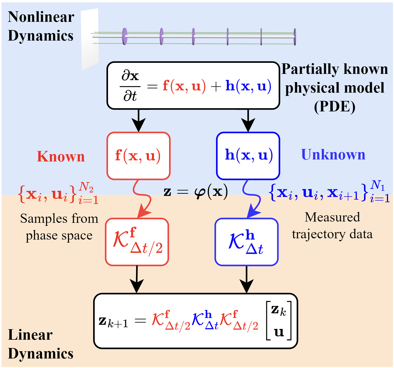
Newtonian mechanics systems, in particular, rely on the principle of superposition, where linear sums of forces determine the dynamics of velocity. Building on this principle, how can we take advantage of this superposition in the case when the form of certain forces are, in general, unknown?

PI-EDMDc looks to take advantage of this, and assumes that governing PDEs can be written in the form

where \(\mathbf{f}\) is a vector field describing the known dynamics of \(\mathbf{x}\), and \(\mathbf{h}\) generically describes the unknown, but linearly separable, terms describing the dynamics of \(\mathbf{x}\).

Slow manifold; nonlinear dynamics with unknown nonlinear forcing

A classical example from literature for Koopman operators is a quadratic slow manifold of two variables

where \(\delta\) is the magnitude of some step impulse applied to the system. \(\mu\) and \(\lambda\) are constants such that when \(u=0\) and \(\vert \lambda \vert \ll \vert \mu \vert\) the system exhibits a slow manifold and a fixed point at the origin.

Importantly, it is known that this system can be embedded into a higher dimensional space \(\begin{bmatrix} y_1 & y_2 & y_3 \end{bmatrix}^\intercal = \begin{bmatrix} x_1 & x_2 & x_1^2 \end{bmatrix}^\intercal\) where the dynamics are linear, namely

Notably, the control input enters the system via a nonlinear function, making the Koopman operator not trivially identifiable by simply choosing the correct dictionary of functions with respect to \(\mathbf{x}\).

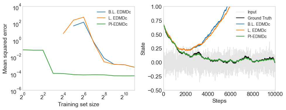
We choose the dictionary of functions \(\Theta(\mathbf{x}, \mathbf{u})\) to be the set of 2nd order monomials. This gives us the following results. PI-EDMDc is capable of taking advantage of the nonlinear known part of the differential equation, reducing the amount of trajectory data needed to learn the unknown term \(\mathbf{h}\).

The left of this figure shows the error as a function of training set size of trajectories. The right shows the performance of each method at a training set size of 2048.

1D heat equation; application to nonlinear partial differential equations

Consider the 1D heat equation with nonlinear forcing, described as

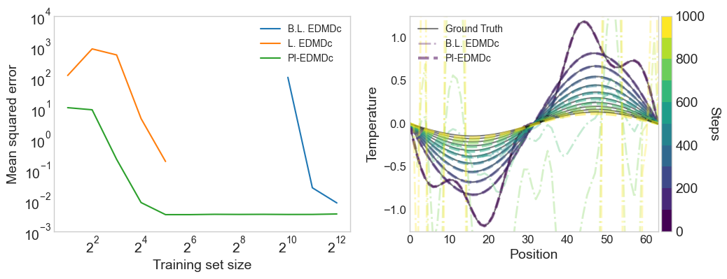
with boundary conditions \(u(0) = u\left( \frac{2\pi}{\alpha} \right) = 0\). If we assume the nonlinear forcing \(\delta \sin(\alpha x)\) to be unknown, but that the passive system of the heat equation is known, then we can learn PI-EDMDc models that take advantage of this. As in the slow-manifold case, PI-EDMDc reduces the amount of true trajectory data required to recover the part of the Koopman operator associated with the unknown the nonlinear forcing.

The left of this figure shows the error as a function of training set size of trajectories. The right shows the performance of each method at a training set size of 1024.

Soft robot; tendon-driven cable actuator

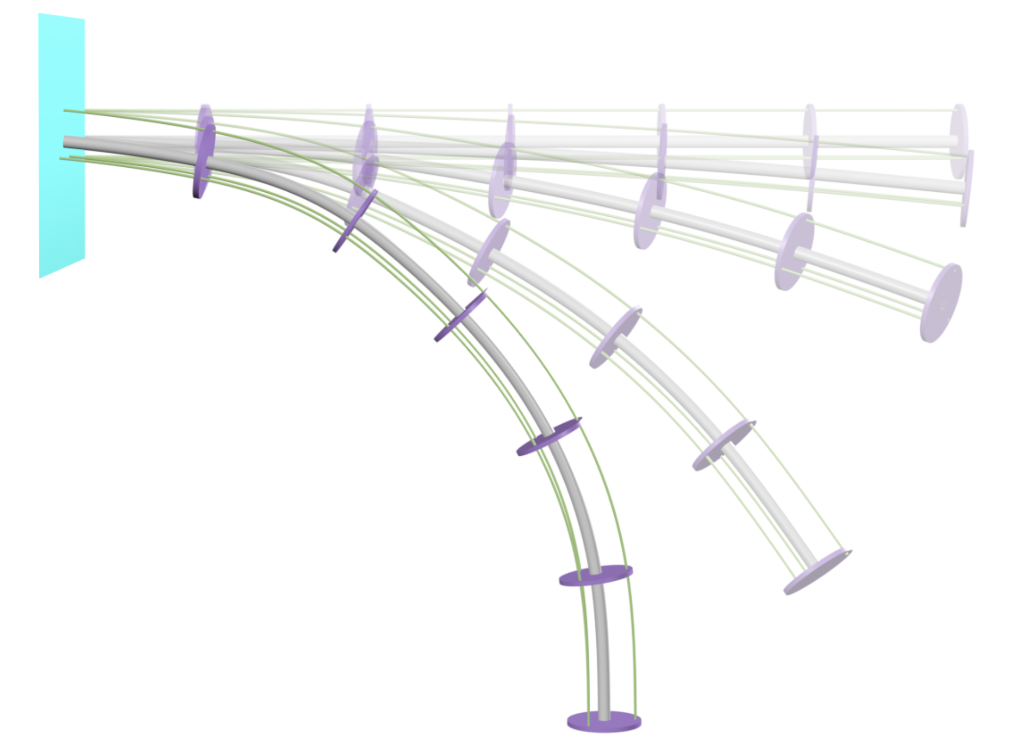
Rendering of a soft robot trajectory

Error of different methods of the position along the backbone (Fig. a and Fig. c). Error of different methods of the velocity at the distal end of the robot (Fig. b and Fig. d).

The governing equations for a soft robotic actuator can be described by the passive dynamics of the backbone, in addition to external forces and actuation forces. The above results are obtained for a simulated soft robot with unknown actuation forces as well as unknown external forces. More information about simulation setup and PDE parameters can be found in the paper.